(Solved): I Have No Idea How To Do This Or Use Excel ...

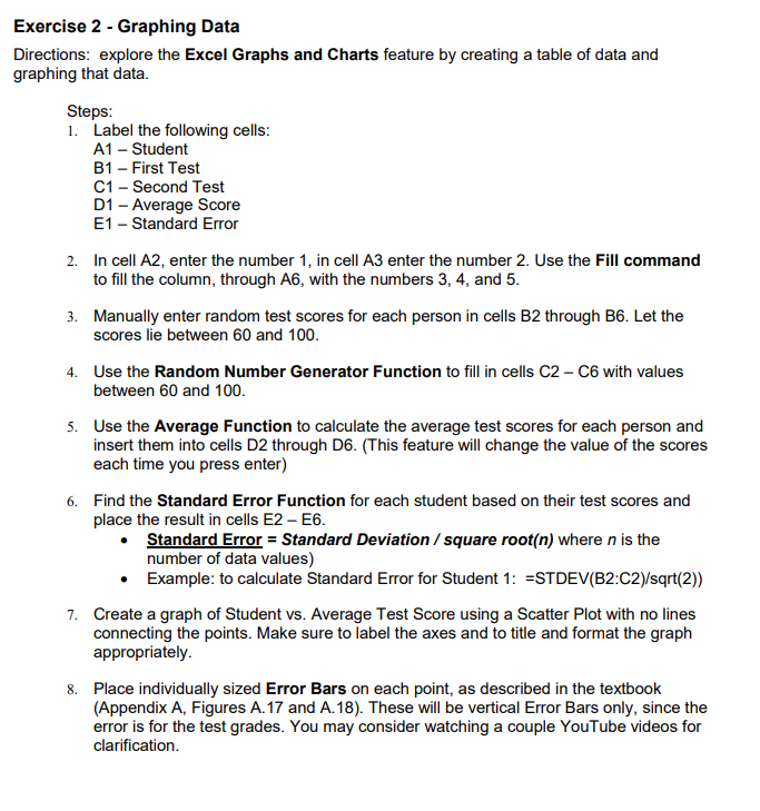
Exercise 2 - Graphing Data Directions: explore the Excel Graphs and Charts feature by creating a table of data and graphing that data. Steps: 1. Label the following cells: A1 - Student B1 - First Test C1 - Second Test D1 - Average Score E1 - Standard Error 2. In cell A2, enter the number 1, in cell A3 enter the number 2. Use the Fill command to fill the column, through A6, with the numbers 3, 4, and 5. 3. Manually enter random test scores for each person in cells B2 through B6. Let the scores lie between 60 and 100. 4. Use the Random Number Generator Function to fill in cells C2-C6 with values between 60 and 100. 5. Use the Average Function to calculate the average test scores for each person and insert them into cells D2 through D6. (This feature will change the value of the scores each time you press enter) 6. Find the Standard Error Function for each student based on their test scores and place the result in cells E2-E6. • Standard Error = Standard Deviation / square root(n) where n is the number of data values) • Example: to calculate Standard Error for Student 1: =STDEV(B2:C2)/sqrt(2)) 7. Create a graph of Student vs. Average Test Score using a Scatter Plot with no lines connecting the points. Make sure to label the axes and to title and format the graph appropriately. 8. Place individually sized Error Bars on each point, as described in the textbook (Appendix A, Figures A. 17 and A. 18). These will be vertical Error Bars only, since the error is for the test grades. You may consider watching a couple YouTube videos for clarification